Harvard-Smithsonian Center for Astrophysics
XRT E2E Test
Day 20050608 Shift B
Test Conductor E. DeLuca
Shift Scientists M. Weber & J. Scott
FOV Optimized Focus Position
Podgorski and Cirtain continued taking data for the FOV-OF sub-test during Shift-A. It was decided that, instead of taking the 1D radial scans at different angles like the previous shift had done, it would be more informative to take 1D "diameter" scans through the p/y = (0,0) position, from -12 to +12 arcmin.
It was also determined that our understanding of the direction of motion of the focus mechanism was reversed, so it became apparent that we needed to move to positions on the positive side of the Best Focus position.
Using the position of Best Focus to be at -850 focus-steps (-515 um), we estimated the focus offset for which the PSF of the optic would be doubled in width. The predicted OF position was -237 focus-steps (-156 um). (The analysis method for predicting the OF position is described in detail in the text file named "fovof_fstep_estimate.txt".)
I show below some plots of the 1D diameter scans at advancing focus positions. First, we note that these results suggest that the optical axis is not aligned to the p/y = (0,0) position, as indicated by the central maxima.
Second, as expected, we see that the central maximum raises as we move towards the OF position. We have defined OF by a threshold value on the observed width of 2.02 pixels. (Yes, the sig-figs are a bit gratuitous.) This threshold is indicated on the plots with a horizontal dashed line. The idea of Optimized Focus is to get as much of the off-axis area below the threshold as we can while keeping the center under the threshold.
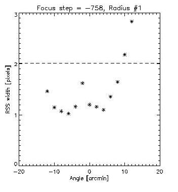
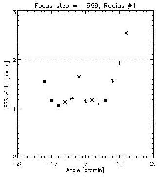
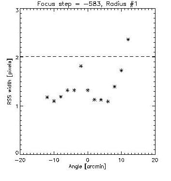
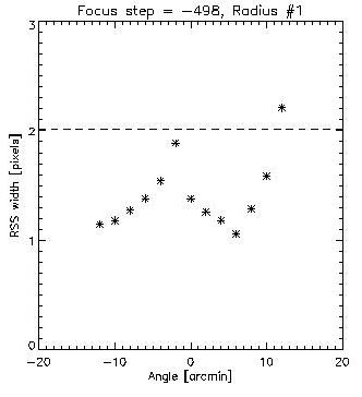
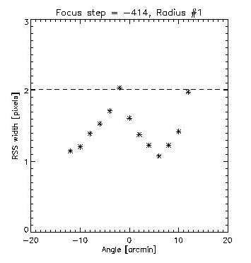
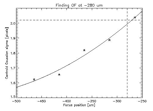
Next, we concern ourselves only with the central peaks of the scans, which we here identify with the optical axis. At what focus position do we cross the OF threshold width?
The next figure is a plot of the centroid widths at the axis as a function of focus position. The OF threshold is again indicated by a horizontal dashed line. We made a conservative estimate of the OF focus position to ensure that we are below the threshold. We end up with OF position = -280 um, which is indicated by a vertical dashed line.
Core PSF at {BF,OF} for source {Cu-L, Al-K}
We did 2D scans in pitch/yaw for two focus positions (BF, OF) using the Cu-L x-ray source. Since we had sufficient time, we repeated the measurements using the Al-K x-ray source. The following plot indicates the positions of the 2D scan measurements.
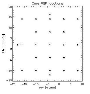
For each measurement, we fitted the image with a Gaussian, and used the sigma as a measure of the spot width. The following plots are contour maps of the spot width across the 2D scans, at the locations displayed above.
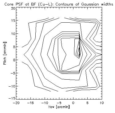
An important note: the scanned locations have some gaps. In order to make the contour map, I replaced the gaps with the maximum data value in the scan. This was done to avoid creating artificial maxima, but it also creates some gradients which are probably exaggerated in comparison to what actual sampling would show.
In the scans at BF position, the contours indicate shallow minima. I think that the "actual" contours around these minima would be reasonably cylindrically symmetric. However, my treatment of coverage gaps probably introduces the sharp corners in the outer sides of the minima's shapes.
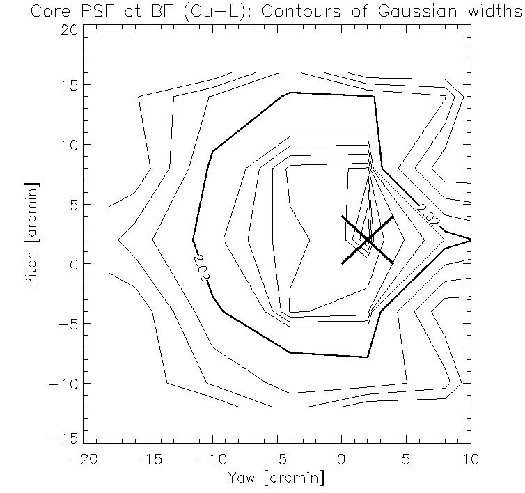
(Subsection: BF, Cu-L)
First, we show plots for the Best Focus position, with the Cu-L source. The first figure shows images of the centroids arranged in their pitch/yaw positions according to the figure above.
The first contour plot shows the distribution of widths again. The second contour plot is a repeat of the the first, with details emphasized. The "2.02" line indicates the optimized FOV (ie, centroid Gaussian sigma < 2.02 pixels). The global minimum is marked with a large "X".
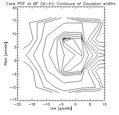
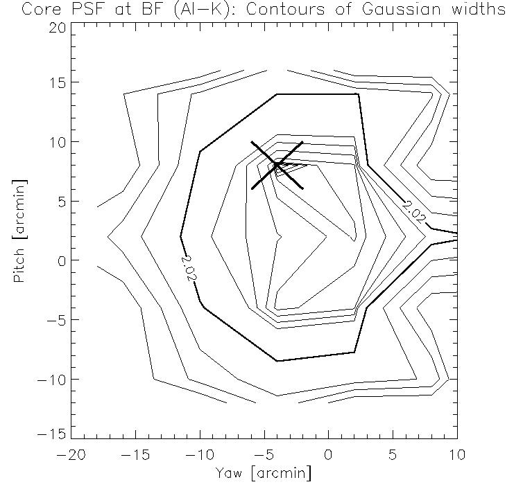
(Subsection: BF, Al-K)
Next, we show plots for the Best Focus position again, this time with the Al-K source. We start again with the mosaic of centroid images. The second contour plot is a repeat of the the first, with details emphasized. The "2.02" line indicates the optimized FOV (ie, centroid Gaussian sigma < 2.02 pixels). The global minimum is marked with a large "X".
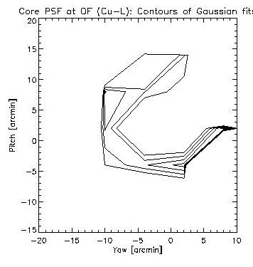
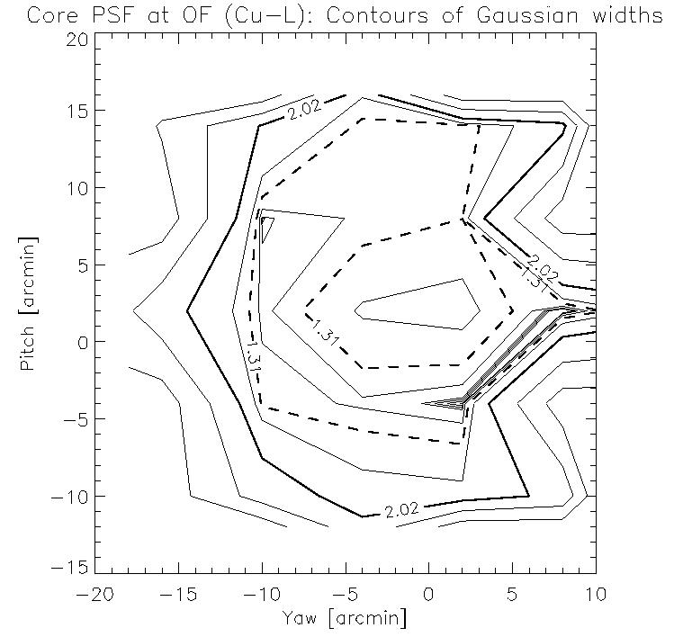
(Subsection: OF, Cu-L)
In the scans at OF position, the contours indicate "C" shaped or "O" shaped valleys (minima). This is expected--- this region corresponds to the bottom of the "W" shapes seen in the FOV-OF plots in the section above. The choice of contour levels to show is tricky. I chose levels to emphasize the "C" shaped valleys. This structure was harder to make out when I tried to contour more of the scanned areas.
The parts of the "C" valleys that extend into the unsampled areas appear to not be part of the minima. As explained above, I think that that is an artifact of the preparation. I would expect the valleys to be "O" shaped if we were to sample that area, too.
Here are the plots for the Best Focus position with the Cu-L source. The second contour plot is a repeat of the the first, with details emphasized. The "2.02" line indicates the optimized FOV (ie, centroid Gaussian sigma < 2.02 pixels). The "1.31" dashed line was chosen to outline the annular valley of minima.
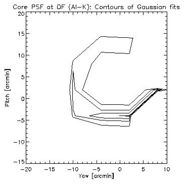
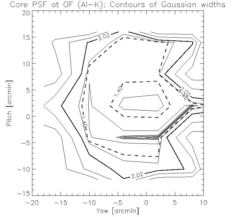
(Subsection: OF, Al-K)
Here are the plots for the Best Focus position with the Al-K source. The second contour plot is a repeat of the the first, with details emphasized. The "2.02" line indicates the optimized FOV (ie, centroid Gaussian sigma < 2.02 pixels). The "1.40" dashed line was chosen to outline the annular valley of minima.